One chart type in Excel that many don’t consider is a scatter plot, also referred to as a scatter graph, scatter diagram, and scatter chart. This type of visual lets you compare two data sets using plotted points. Microsoft Excel provides a handful of scatter plot types depending on how you want to display your data. Let’s have a look at each one and how to create the scatter chart in Excel.
Scatter Chart Types in Excel
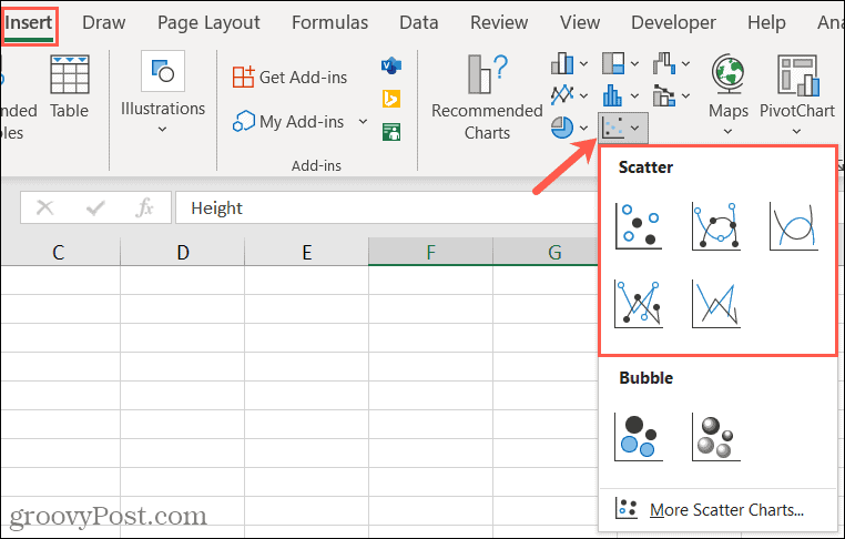
You can select from five different scatter plots with and without markers.
Scatter with markersScatter with smooth lines, with or without markersScatter with straight lines, with or without markers
You’ll also notice in the Scatter Chart menu options for bubble and 3-D bubble charts. While similar to scatter charts, bubble charts use an additional number field to determine the sizes of the data points.
Create a Scatter Plot in Excel
If you have your data sets and want to see if a scatter plot is the best way to present them, it takes only a few clicks to make the chart. Select the data for your chart. If you have column headers that you want to include, you can select those as well. The chart title will default be the header for your y-axis column. But you can change the title for the chart either way.
Go to the Insert tab and click Insert Scatter or Bubble Chart in the Charts section of the ribbon. If you’re using Excel on Windows, you can put your cursor over the various scatter chart types to see a brief description and a preview of the chart.
When you see the chart you want to use, click to insert it into your spreadsheet. You can then select the chart to drag it to a new spot or drag it from a corner to resize it.
Customize the Scatter Chart
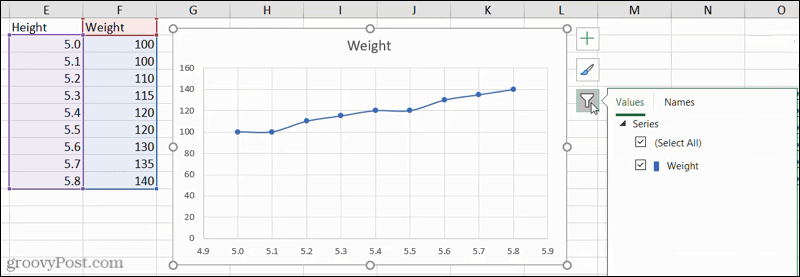
Also, with the chart selected, you’ll see a few buttons displayed to the right. Use these to edit the Chart Elements, Styles, or Filters. Chart Elements: Adjust the titles, labels, gridlines, legend, and trendline.
Chart Styles: Choose a different chart style or color scheme.
Chart Filters: Filter the data to display using values or names.
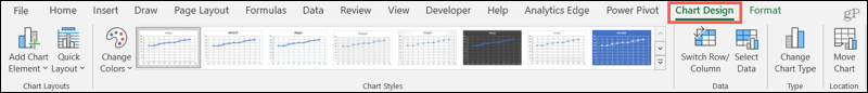
You can also use the Chart Design tab that displays when you select your chart. You can add elements, change the colors or style, switch the rows and columns, or change the chart type.
Include a Third Data Set to the Scatter Plot
Because Excel does a great job at providing scatter plot options that use color, you can add another data set to your chart. Using the same type of scatter plot with smooth lines and markers, you can see here how the chart displays when selecting three data sets.
Plot Your Data With a Scatter Chart in Excel
The next time you want a graphic display of your data and have just a couple of data sets, consider a scatter plot in Excel. It might just be the ideal visual for your spreadsheet. For more, take a look at how to create a Gantt chart in Excel. Or, for something on a smaller scale, check out how to use sparklines in Excel. Comment Name * Email *
Δ Save my name and email and send me emails as new comments are made to this post.


![]()
